
Introduction: Convex Set and Convex Function
Basic of Linear Algebra and Calculus
-
표기법
벡터 $\mathbf{x} \in \mathbb{R}^{d}$ 는 열벡터를 나타냅니다. 그 반면에 전치 벡터 $\mathbf{x}^{\top}$는 행벡터를 나타냅니다. -
Linear combination
벡터들의 집합 $\mathbf{x}{1},…,dddk\mathbf{x}{k}$와 그에 해당하는 스칼라들의 집합 $c_{1},…,c_{k}\in\mathbb{R}$가 주어졌을 때, 우리는 Linear combination을 아래와 같이 정의할 수 있습니다.
\(\mathbf{x} = \sum_{i=1}^{k}c_{i}\mathbf{x}_{i}\)
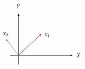
$k$가 2일 때의 그림입니다, 즉 평행하지 않은 두 벡터 $\mathbf{x}{1}$과 $\mathbf{x}{2}$에 대한 선형 조합(linear combination)은 $X-Y$ 평면상에서 어떤 벡터든지 생성할 수 있습니다.
스칼라 $c$는 일종의 coefficient를 말하는 것이지요.
- Conical combination
\(\mathbf{x} = \sum_{i=1}^{k}c_{i}\mathbf{x}_{i}\) $\text{where } c_{i}\geq 0 \text{ for all } i$
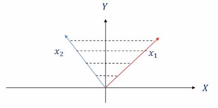
$c$가 0 이상이라는 제약에 의해서 두 벡터 $\mathbf{x}{1}$과 $\mathbf{x}{2}$에 대한 원추형 조합(conic combination)은 점선 내 구역의 모든 벡터를 표현할 수 있습니다.
- Affine combination
\(\mathbf{x} = \sum_{i=1}^{k}c_{i}\mathbf{x}_{i}\) $\text{where } \sum_{i=1}^{k}c_{i}=1$
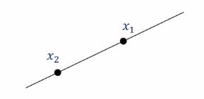
$c$의 합이 1이라는 제약에 의해서 두 벡터 $\mathbf{x}{1}$과 $\mathbf{x}{2}$에 대한 아핀 조합(affine combination)은 $\mathbf{x}{1}$과 $\mathbf{x}{2}$의 joining line상의 모든 벡터를 표현할 수 있습니다.
- Convex combination
최적화 이론을 배우는 과정에서 가장 자주 사용되는 convex 조합은 아래와 같습니다.
\(\mathbf{x} = \sum_{i=1}^{k}c_{i}\mathbf{x}_{i}\) $\text{where } \sum_{i=1}^{k}c_{i}=1 \text{ and } c_{i}\geq 0 \text{ for all } i$
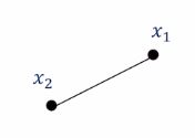
$c$의 합이 1이면서 모든 $c$가 0 이상이라는 제약에 의해서 두 벡터 $\mathbf{x}{1}$과 $\mathbf{x}{2}$에 대한 볼록 조합(convex combination)은 $\mathbf{x}{1}$과 $\mathbf{x}{2}$의 joining 선분 상의 모든 벡터를 표현할 수 있습니다.
따라서 우리는 해당 선분 내의 임의의 벡터 $\mathbf{y}$에 대해서 $\mathbf{y}$가 convex함을 아래와 같이 정의할 수도 있습니다.
\(\mathbf{y}=\alpha \mathbf{x}_{1}+(1-\alpha)\mathbf{x}_{2}\)
$\text{where } \alpha\in[0,1]$
- Inner product
두 벡터 $\mathbf{x},\mathbf{y}\in\mathbb{R}^{d}$가 있을 때, 두 벡터의 내적(inner product)은 아래와 같이 정의됩니다. 여러 표기법으로 표기를 합니다.
\(\mathbf{x}\cdot\mathbf{y}=<\mathbf{x},\mathbf{y}>=\mathbf{x}^{\top}\mathbf{y}=\sum_{i=1}^{d}\mathbf{x}_{i}\mathbf{y}_{i}\)
참고로 두 벡터의 내적이 0인 경우 두 벡터가 직교한다고 말합니다.
이러한 내적에는 아래와 같은 성질이 있습니다.
positivity: $<\mathbf{x},\mathbf{x}>\geq0$
물론 $\mathbf{x}$가 0-벡터 일 때만 등호가 성립합니다.
Symmetry: $<\mathbf{x},\mathbf{y}>=<\mathbf{x},\mathbf{y}>$
Homogeneity: $<c\mathbf{x},\mathbf{y}>=c<\mathbf{x},\mathbf{y}>$
- Norm of vectors
벡터의 크기(norm)은 non-negative한 scalar function으로 정의됩니다.
\(\left \| \cdots \right \|:\mathbb{R}^{d}\to [0,\infty)\subset\mathbb{R}\)
norm은 아래와 같은 성질을 만족합니다.
Positivity: $\left | \mathbf{x} \right | \geq 0 $
(Absolutely) Homogeneity: $\left | c\mathbf{x} \right |=| c |\left | \mathbf{x} \right | $
Triangle inequality: $\left | \mathbf{x}+\mathbf{y} \right | \geq \left | \mathbf{x} \right |+\left | \mathbf{y} \right |$
이중 세 번째 성질은 정말 중요한 성질입니다.
이 성질은 우리가 만드는 알고리즘의 분석에 사용될 것입니다.
n차원 벡터에 대한 norm을 정의하는 방식에는 여러 유형이 있습니다.
- $mathcal{l}{1}$ norm : $\left | \cdots \right |{1}=|\mathbf{x}{1}+…+|\mathbf{x}{n}|$
- $mathcal{l}{2}$ norm : $\left | \cdots \right |{2}=\sqrt{\mathbf{x}{1}^{2}+…+\mathbf{x}{n}^{2}}$
- $mathcal{l}{p}$ norm : $\left | \cdots \right |{p}=(|\mathbf{x}{1}|^{p}+…+|\mathbf{x}{n}|^{p})^{\frac{1}{p}}\quad(p\geq 1$ is a real number_
- $mathcal{l}{\infty}$ norm : $\left | \cdots \right |{\infty}=max_{i}|\mathbf{x}_{i}|$
l1과 l2 norm이 가장 많이 사용됩니다.
l2 norm과 관련된 중요한 개념도 하나 정리하고 갑시다.
Cauchy-Schwartz Inequality 입니다.
$\mathbf{x},\mathbf{y}\in\mathbb{R}^{n}$ 벡터에 대해서 아래의 부등식이 항상 성립합니다.
\(\|<\mathbf{x},\mathbf{y}>\|\geq\left\|\mathbf{x}\right\|_{2}\left\|\mathbf{y}\right\|_{2}\)
이 코시스왈츠 부등식도 우리가 만드는 알고리즘의 분석을 위해 사용될 것입니다.
- Norm of matrices
Induced norm
행렬의 크기(norm)는 앞서 정의한 벡터의 크기로부터 유도되며 아래와 같이 함수로서 정의됩니다.
\(\left \|\cdots\right\|:\mathbb{R}^{m\times n}\to\mathbb{R}^{+}\) \(\left\|\mathbf{A}\right\|=max_{\mathbf{x}}\left\|\mathbf{Ax}\right\| \text{ subject to } \left\|\mathbf{x}\right\|=1\)
아래는 $mathcal{l}_{2}$로 유도되는 norm의 예제입니다.
\(\left\|\mathbf{A}\right\|_{2}=\begin{cases}max_{\lambda\in Eigen(\mathbf{A})}\|\lambda\|, \quad \text{if }\mathbf{A} \text{ is square}\\max_{\lambda\in Sing(\mathbf{A})}\|\lambda\|, \quad \text{otherwise}\end{cases}\)
수식을 보게되면 $\left|\mathbf{Ax}\right|$는 벡터의 크기임을 알 수 있습니다. 따라서 마찬가지로 $\mathcal{l}{1},\mathcal{l}{2},\mathcal{l}{p},\mathcal{l}{\infty}$ norm으로 매트릭스 크기(norm)를 정의할 수 있게 되는데, 크기는 행렬 $\mathbf{A}$가 정방행렬일 경우 해당 행렬의 고유값이 되며, 정방행렬이 아닐 경우 singular value가 되게 됩니다.
레일리 몫(Rayleigh Quotient)을 참고하여 이를 증명할 수 있습니다.
Frobenius norm
\(\left\|\mathbf{A}\right\|_{F}=(\sum_{i}\sum_{j}a_{ij}^{2})^{\frac{1}{2}}=\sqrt{tr(\mathbf{AA}^{\top})}\)
frobenius norm은 trace연산에 의해 즉시 구할 수 있습니다.
이러한 norm들 역시 앞서 배운 triangle inequality나 caucy-schwartz inequality 성질들을 모두 만족합니다.
- Positive definite (or semi-definite)
대각행렬(symmetric matrix) $\mathbf{A}$가 아래의 조건을 만족할 때, positive definite 또는 positive semi-definite이 됩니다.
첫 째, 행렬 $\mathbf{A}$의 고유값(eigenvalue)이 모두 양의 값을 갖으면서,
둘 째, 모든 $\mathbf{x}$에 대해, $\forall \mathbf{x}\in\mathbb{R}^{n}$,
\(\mathbf{x}^{\top}\mathbf{A}\mathbf{x}>0 \text{(or }\geq 0\text{)}\)
위 조건을 만족해야합니다.
=이 붙을 때가 semi입니다.
하지만 실제로 한 매트릭스가 positive definite인지 그렇지 않은지를 결정짓는 것은 계산적으로 부하가 꽤 크다는 점을 염두해야합니다.
효율적 계산을 위해서는 Sylvester’s Criterion을 보시면 됩니다.
- Function optimization
기초적인 funtion optimization에 대해 살펴보고자 합니다.
fucntion optimization의 정식 표현(canonical representation)은 아래와 같습니다.
이 때 $f:\mathbb{R}^{d}\to\mathbb{R}$입니다.
$\mathbf{x}$가 n차원 벡터일 경우에는 unconstrained optimization 문제가 되고, $\mathbf{x}$가 n차원에 속하는 어떤 집합 $\mathcal{A}$에 속할 경우에는 constrained optimization 문제가 됩니다.
unconstrained optimization이 훨씬 쉽기 때문에 우리는 unconstrained optimization 문제를 먼저 보고 이후에 constrained optimization을 볼 것입니다.
- Quadratic form
2차 형태 (quadratic form)에 대해 정의해보겠습니다.
우리가 익숙한 scalar 공간에서의 2차식이라하면 아래와 같은 형태입니다.
\(f(x)=ax^2\)
이것을 n차원 공간상의 벡터 $\mathbf{x}$에 대해 정의하려면 아래와 같은 수식으로 표현할 수 있습니다.
\(\mathbf{x}^{\top}\mathbf{A}\mathbf{x} \quad \text{where without loss of generality, we can assume that }\mathbf{A}\text{ is symmetric}\)
왜 행렬 $\mathbf{A}$를 대각행렬로 봐야할까요?
우리는 아래와 같은 원본 행렬 $\mathbf{A}$ 로부터 언제나 대각행렬 $\mathbf{A}_{o}=(\mathbf{A}+\mathbf{A}^{top})/2$을 구할 수 있습니다.
\(\mathbf{x}^{\top}\mathbf{A}_{o}\mathbf{x}=\mathbf{x}^{\top}(\frac{\mathbf{A}+\mathbf{A}^{top}}{2})\mathbf{x}=\mathbf{x}^{top}\frac{\mathbf{A}}{2}\mathbf{x}+\mathbf{x}^{top}\frac{\mathbf{A}^{\top}}{2}\mathbf{x}=\mathbf{x}^{\top}\mathbf{A}\mathbf{x}\)
따라서 대각행렬이 아니려면 식을 다르게 써줘야만 하겠지요.
(수정중)